Everything happens somewhere.

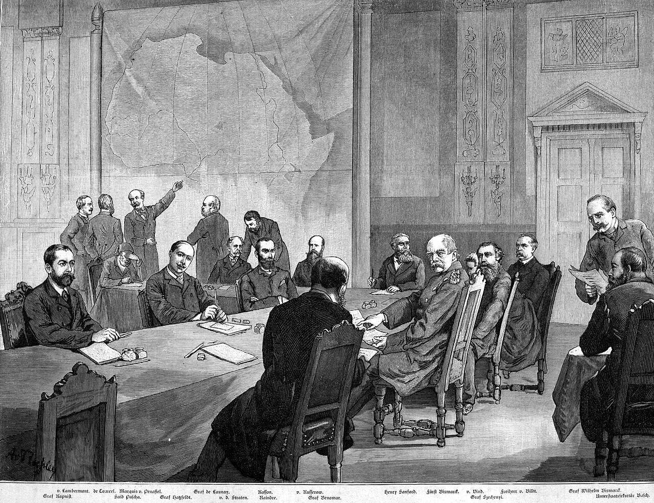
In the engraving the map hangs on the wall behind the table, and a delegate stands and points at it. Between 15 November 1884 and 26 February 1885, representatives of fourteen states met in Berlin at the invitation of Otto von Bismarck to agree the rules for dividing Africa among European powers, and no African state was invited. The lines that followed over the next decades were drawn far from Africa by people with little knowledge of who lived where, and many of them still stand.

Historians of Africa have long argued that these borders did lasting harm. A line that cuts through an ethnic group’s homeland can leave its members agitating to rejoin their kin on the other side, and gives armed groups somewhere to retreat across it. The argument is plausible, but for a century it was hard to test systematically. The evidence sat in different maps, made by different people for different purposes. What made the test possible was software for laying one map on top of another.

In this article, which became the methods chapter of my dissertation, I introduce that software, geographical information systems, to political scientists. I make three claims:

• Almost everything political scientists study has a location.
• Location is a key that can join data that otherwise have nothing in common.
• Joining data by location makes new research designs possible, including designs that avoid a trap built into comparisons of countries.

The Scramble for Africa is the article’s running example, and I use it here too, along with the maps I made for the dissertation’s other chapters.

Modern political science has mostly taken two things as its natural units: sovereign states and the individuals inside them. Does economic development lead to democracy? Correlate income per head with democracy across as many countries as possible, over as many years as possible. Does education make people more tolerant? Survey as many individuals as possible. International relations was built on the premise that relations between sovereign states hold the key to war and peace.

It was not always like this: the founders of academic political science in the United States, at Johns Hopkins University in the late nineteenth century, studied how ideas and institutions spread across territory, and the tradition produced Frederick Jackson Turner’s thesis about the American frontier. The behavioural revolution, with its national statistics and representative surveys, pushed geography out of the mainstream.

The older work was often rich and suggestive, but weaker at ruling out alternative explanations than the quantitative work that replaced it. A few classics kept place at the centre: V. O. Key’s Southern Politics in State and Nation (1949), Robert Dahl’s Who Governs? (1961) and Robert Putnam’s Making Democracy Work (1993).

By the 2010s the two units were under pressure from several sides. Students of the European Union pointed out that authority was moving upwards and downwards from the state. Africanists and others noted that many governments do not control all of their own territory. Studies of political behaviour found that neighbours and social networks shape how people vote. Methodologists questioned both methodological individualism and methodological nationalism.

The risk in this kind of criticism is that it ends in a shrug: politics is complicated, and everything depends on context. My proposal in the article is narrower. Cultivate what I called spatial awareness, always trying to locate politics in space, and use the tools that make location usable. The starting premise is that almost every kind of information has a geographical referent.

A geographical information system stores data as layers, each tied to coordinates on the earth’s surface. There are four basic kinds:

• Points are single locations: a church, a battle, the home of a survey respondent.
• Lines connect points: a road, a river, a pipeline.
• Polygons are lines that close on themselves around an area: a country, a province, a lake.
• Rasters are grids that hold a value for every cell, such as altitude, temperature, or the light that settlements emit at night, which satellites record and which researchers use as a measure of income in Africa.

Simply putting data on a map already helps. Gary King made the point in 1996: displaying data geographically connects a variable with many others measured for the same places, and most readers know the values of many of those without looking them up. In 2016, Harvard’s free WorldMap platform let anyone stack slave ports, rivers, ethnic groups and religious composition on one map of Africa with a few clicks. The figure below builds a similar stack from the dissertation’s own data and from Natural Earth, a free public collection of map layers.

Joining layers is the basic operation, and these are the main kinds. If the unit of analysis is a polygon, such as a province, one can count the points inside it (battles in a civil war, say), record whether a line crosses it (a road or a river), average a raster over it (altitude, night lights), or measure how much of it overlaps with other polygons (parliamentary constituencies).

If the unit is a point, such as a survey respondent’s home, it can take on the attributes of the polygon it lies in (the soil type of the district), its distance to a line (a border, a highway), the average of a raster around it (night lights within 25 kilometres), or its distance to other points (the nearest school).

I used most of these joins in the dissertation, and three of them follow.

Each of these joins made a comparison possible that tables alone could not. In the Africa chapter, placing oil and gas fields inside regions showed something that country statistics hide. Between countries, oil and Islam go together, because so many Muslim-majority states export petroleum. Between regions, they are almost unrelated, with a correlation of 0.06. That is what allowed me to separate the two explanations.

The general point is that location is a common denominator of almost all data, so datasets whose units do not match can often be made to match by adding coordinates. Historical sources, such as lists of towns, census records and old borders, can often be geocoded cheaply, and many newer sources, such as search queries and social media posts, already carry locations.

My main example in the article is a study by the economists Stelios Michalopoulos and Elias Papaioannou of the long-run effects of the Scramble for Africa, then forthcoming and since published in the American Economic Review. It shows what the four kinds of data can do together. In the steps below the shapes are a diagram; the numbers are the study’s.

The study then links layers that were never designed to fit together. Matched to the Ethnic Power Relations dataset, which was not geocoded, partitioned groups turn out to be more likely to suffer discrimination by their governments and to be involved in ethnic civil wars. Government forces, rebels and militias, and above all foreign government forces, are more active in partitioned areas, which fits accounts of states invading neighbours to protect kin across the border.

Household surveys with locations, from the Demographic and Health Surveys, add individuals. Members of partitioned groups have lower living standards, less access to running water and electricity, and less education, and this holds wherever they live, inside or outside their group’s homeland. Members of other groups who live in partitioned areas are not worse off, and partitioned areas are no poorer in the night lights seen from space. The disadvantage travels with the members of split groups.

My reading in 2016 was that historians of Africa had largely been right about borders and violence, while the economic damage fell on members of the split groups rather than on whole regions. The study also left questions that only more spatial work could answer. It used today’s borders and did not trace how they changed after 1884. Which borders moved, and were those that split groups more likely to move later?

Spatial data do more than add variables. They change which comparisons are possible, and that matters for a problem that comparisons of countries cannot escape on their own.

Geographers call it the modifiable areal unit problem. When local data are summarised into larger units, the summaries depend on where the boundaries are drawn whenever the variable differs from place to place. Political scientists who study gerrymandering know the phenomenon well: move the district lines, and the same voters elect different representatives.

For comparisons of countries the problem has a sharp edge. The number of states and the lines between them are themselves outcomes of politics: of colonisation, state capacity, federalism, secession, war and peace. Whenever the variables in a cross-country study also helped to make or unmake states, the units themselves can bias the result. The figure below shows how much the choice of units can matter, using the regional data from the Africa chapter.

None of these numbers is wrong. Each describes a different set of units, and only some of those units were drawn by anyone with a stake in the answer.

In the article I apply the same worry to the Scramble for Africa study, which is mostly a comparison within countries. If partition or civil war affected how many states emerged and where their borders came to lie, the estimates are biased, which seems likely, since Africa’s two newest states, Eritrea and South Sudan, both emerged from vicious civil wars with ethnic dimensions. If borders have since moved away from conflict-prone areas and towards ethnic boundaries, groups that are still partitioned today may see less conflict than partition originally caused, and the study’s estimate would be too small.

Spatial tools also offer remedies. The analysis can be repeated using only borders that have not changed since 1885, since 1914 or since 1960. Or it can be run on virtual countries, grids whose boundaries no politics drew.

In comparative politics, studies of party systems, ethnic relations, public goods, multilevel government and election fraud informed by geography were beginning to appear when I wrote the article. I cite Nahomi Ichino and Noah Nathan on local ethnic geography and voting in Ghana, and Peter Thisted Dinesen and Kim Mannemar Sønderskov on ethnic diversity and trust in people’s immediate surroundings. In international relations, a 2014 special issue of the Journal of Conflict Resolution on joining micro and macro approaches to civil war signalled a spatial turn.

Public administration was the odd one out, because governments use these tools constantly, to decide where to build schools, hospitals and roads and to manage the services they already run. The New York Times described in 2013 how New York City’s policy office under Mayor Michael Bloomberg relied on spatial data. Yet research on public administration, including its large literature on networks of agencies and officials whose ties depend on distance, had barely used them.

I end the article with theory. Thinking spatially can bring into view political phenomena that a focus on countries and individuals hides, and it can tie the levels of politics together: local officials, regional governments, national leaders and international actors, and the links between places at the same level.

For the Scramble for Africa, that means asking how local officials stoke or damp conflict, how local government shapes ethnic inequality, what national governments want from local outcomes, and how subnational boundaries are drawn. After 1994 Ethiopia redrew its regions around its large ethnic groups, including a Somali regional state in the east, which gave regional leaders resources that could be used in conflict. Ethiopian–Somali conflict flared from 1998 to 2003 and again from 2006 to 2009.

This chapter is the method behind the others. The dissertation asks how culture and institutions shape each other, and each of its designs depends on places: a border that moved twice across the same towns, regions that share a national state but not a religion, immigrants who carry one country’s habits into another. Most of them needed a map to define who had been exposed to what.

Geography has been studied by historians, area specialists and qualitative researchers since political science began. The tools let quantitative researchers test their accounts systematically, and give qualitative researchers another source of evidence. Maps can be a place where the two kinds of research meet.